My first neural network classifier, statue or painting?
Recently I decided to learn deep learning and the math behind the training process and I’d like to summarize what I’ve learned so far by writing a simple but efficient classifier, a neural network capable to tell if an image contains a painting or a statue.
The code uses FastAI deep learning library, mainly because of their motto FASTAI: Making neural nets uncool again and I used Colab, a cloud Python editor with GPU support, to write the code.
Table of Contents #
- Table of Contents
- Prepare the dataset
- Install the libraries
- Configure the datasets
- Train the architecture into a model
- Testing the neural network
- Conclusions
Prepare the dataset #
Last week I went to the Uffizi Museum and I toke some pictures of paintings and statues so I decided to use them as my training data.
I removed the blurred photos and split them into two folders, named paint and statue, the folder name is very important because the training code uses it to label the content.
Install the libraries #
The first lines of code are for installing libraries and importing the necessary modules.
!pip install fastai==2.2.5
!pip install exif

from fastai.data.all import *
from fastai.vision.all import *
from exif import Image as ExifImage
An issue I had is that fastai by default doesn’t rotate the images according to their EXIF metadata so I searched and found a piece of code to rotate the photos in the correct orientation before feeding the neural network with them.
def exif_type_tfms(fn, cls, **kwargs):
  def get_orientation(fn: (Path, str)):
    with open(fn, 'rb') as image_file:
      exif_img = ExifImage(image_file)
      try:
        return exif_img.orientation.value
      except AttributeError:
        # ignore orientation unset
        return 1
  def f(img, rotate=0, transpose=False):
    img = img.rotate(rotate, expand=True)
    if transpose:
      img = img.transpose(Image.FLIP_LEFT_RIGHT)
    return img

  # Image.rotate will do shorcuts on these magic angles, so no need for any
  # specific resampling strategy
  trafo_fns = {
    1: partial(f, rotate=0),
    6: partial(f, rotate=270),
    8: partial(f, rotate=90),
    3: partial(f, rotate=180),
    2: partial(f, rotate=0, transpose=True),
    5: partial(f, rotate=270, transpose=True),
    7: partial(f, rotate=90, transpose=True),
    4: partial(f, rotate=180, transpose=True),
  }
  img = cls.create(fn, **kwargs)
  orientation = get_orientation(fn)
  img = trafo_fns[orientation](img)
  return cls(img)

def ExifImageBlock(cls=PILImage):
  """
  if images are rotated with the EXIF orientation flag
  it must be respected when loading the images

  ExifImageBlock can be pickled (which is important to dump learners)
  >>> pickle.dumps(ExifImageBlock())
  b'...
  """
  return TransformBlock(type_tfms=partial(exif_type_tfms, cls=cls), batch_tfms=IntToFloatTensor)
Configure the datasets #
datablock = DataBlock(
    get_items=get_image_files, # how to gather images
    item_tfms=Resize(224), # how to transform images before use them
    blocks=(ExifImageBlock, CategoryBlock), # (input transforms, label transforms)
    get_y=parent_label, # how to label the images
    splitter=RandomSplitter()) # how to get the training dataset
A DataBlock represents a list of instructions used by the network to gather the dataset, label it, transform it, and how to split it into a training dataset and a validation dataset.
The get_image_files function is a utility that grabs all the files in a folder, recursively.
The Resize function resizes the image to 224px x 224px. Why 224px? It’s a standard size, you can use the value you’d like but remember that a larger image requires more resources to be processed.
The blocks attribute is a Tuple that contains the block of the x, our input dataset, and the block of the y, our labels.
A block represents a set of transformations to apply.
The ExifImageBlock will rotate the images according to the EXIF metadata, and the CategoryBlock indicates that images are labeled with only two categories, in my case statue or paint.
The parent_label function receives the image path as input and returns the name of the containing folder, my label.
So if the photo of a statue is inside the statue folder, the neural network will learn that that photo is a statue.
The RandomSplitter() without any parameters will create a validation dataset using 20% of the input dataset.
dls = datablock.dataloaders('/content/drive/MyDrive/uffizi', bs=5)
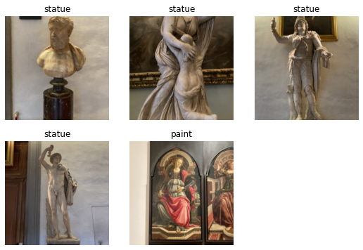
dls.show_batch()
The bs attribute is the batch size, how many training examples the neural network will process at a time. The larger the batch size the more resources you need, the smaller the batch size the more updates you need.
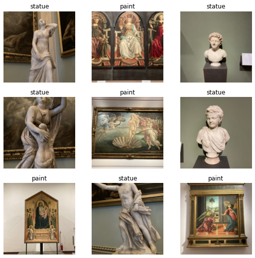
The show_batch method shows the first batch that the neural network will process.
All the images are labeled with their parent folder name.
Train the architecture into a model #
learn = cnn_learner(dls, resnet34, metrics=error_rate)
learn.fine_tune(4)
Here we use a convolutional neural network, inspired by biological processes, is the state-of-the-art in image recognition, NPL, and bioinformatics.
resnet34 is a Residual Network, a model pre-trained with the ImageNet dataset, it consists of 34 layers.
The fine_tune(4) call will train the neural network with our dataset 4 times, each time is called epoch.
For each epoch, it tests the goodness of the model using the validation dataset by calculating the loss value.
Looking at the output of the training process we notice an issue, from the 2nd epoch to the 4th epoch the loss is increasing meaning that the model is getting worse, the learning process is not working correctly, and the reason for that is the batch size and how it interferes with the SGD (Stochastic Gradient Descent), that is not completely clear to me why it happens but I’ll investigate more and I’ll write a post about it.
| epoch | train_loss | valid_loss | error_rate | time |
|---|---|---|---|---|
| 0 | 0.774661 | 0.121791 | 0.071429 | 00:38 |
| epoch | train_loss | valid_loss | error_rate | time |
|---|---|---|---|---|
| 0 | 0.187633 | 0.038042 | 0.000000 | 00:49 |
| 1 | 0.109573 | 0.007019 | 0.000000 | 00:49 |
| 2 | 0.356412 | 0.003473 | 0.000000 | 00:49 |
| 3 | 0.373253 | 0.004066 | 0.000000 | 00:50 |
Let’s increase the batch size to 10 and re-launch the training.
datablock = DataBlock(
    get_items = get_image_files,
    item_tfms=Resize(224),
    blocks=(ExifImageBlock, CategoryBlock),
    get_y=parent_label,
    splitter=RandomSplitter())
dls = datablock.dataloaders('/content/drive/MyDrive/uffizi', bs=10)
dls.show_batch()
learn = cnn_learner(dls, resnet34, metrics=error_rate)
learn.fine_tune(4)
With a batch size value of 10 the loss decreases for each epoch as we expected, our network is learning!!!
| epoch | train_loss | valid_loss | error_rate | time |
|---|---|---|---|---|
| 0 | 0.852532 | 0.558232 | 0.214286 | 00:37 |
| epoch | train_loss | valid_loss | error_rate | time |
|---|---|---|---|---|
| 0 | 0.359626 | 0.068505 | 0.000000 | 00:46 |
| 1 | 0.293746 | 0.003416 | 0.000000 | 00:46 |
| 2 | 0.260396 | 0.004584 | 0.000000 | 00:46 |
| 3 | 0.192967 | 0.005092 | 0.000000 | 00:46 |
A confusion matrix is helpful to understand where our neural network is wrong, we can print it using the following code.
interp = ClassificationInterpretation.from_learner(learn)
interp.plot_confusion_matrix()
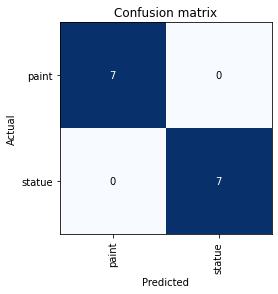
Nothing wrong so far 🚀
Testing the neural network #
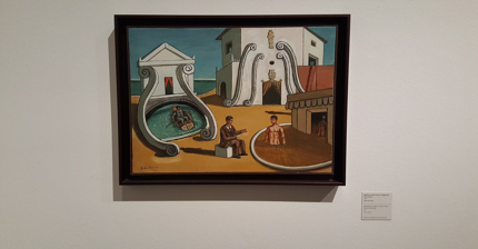
Now we create an image object using a painting that the model has never seen.
Using an image that the network has never seen is very important, you can’t test the network with the images contained in your input dataset, it’s cheating if you do that.
paint = PILImage.create('/content/dechirico1.jpg')
paint = PILImage(paint.resize((430, 224)))
paint
learn.predict(paint)
('paint', tensor(0), tensor([0.9841, 0.0159]))
Hurray!!! The network has confidently classified the image as a painting, it’s 98.41% sure about that. Let’s try with another painting that contains a statue 🙄
paint = PILImage.create('/content/dechirico2.jpg')
paint = PILImage(paint.resize((224, 224)))
paint
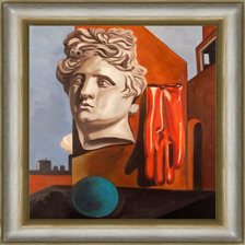
learn.predict(paint)
('paint', tensor(0), tensor([0.9972, 0.0028]))
It’s 99% sure about paint category 🎉
And finally lady liberty.
paint = PILImage.create('/content/ladyliberty.jpg')
paint = PILImage(paint.resize((224, 224)))
paint
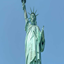
learn.predict(paint)
('statue', tensor(1), tensor([0.0070, 0.9930]))
It’s 99% sure that it is a statue 🗽
Conclusions #
I am amazed how with so few images it’s possible to create a neural network to classify images that have never been seen by the training process.
One of the most important things to get a good result is to have a good training dataset and a good dataset for validation, the organization of the input dataset is crucial to have a good model capable of making predictions.
Deep learning is not just for image recognition, it can be applied to almost all fields, including natural language processing, bioinformatics, recommendation systems, etc.
I’m still just scratching the surface of deep learning, there are so many things to learn, I’ll continue to study it and to write about it.